Up: Issue 5
Next: Paper 2
Voting matters - Issue 5, January 1996
Estimating the Probability of Monotonicity Failure in a UK General
Election
Dr C Allard
Crispin Allard holds a PhD in statistics from the University of Warwick,
and is a member of the ERS Council.
1. Summary
Three years ago, the Plant Report rejected STV as a system worth considering
for elections to the House of Commons, citing evidence submitted by Michael
Dummett (based on an example originating from Reference
[2]) on the grounds that it could be non-monotonic. In this paper I
attempt to estimate the probability of a monotonicity failure which affects
the number of seats won by a party. I estimate the probability of this
occurring in a multi-member constituency in one election as: 2.5 ×
10**(-4), equivalent to less than once every century across the whole UK.
[This result was first reported in Reference [1] as 2.8
× 10**(-4). I have revised this down as a result of a refinement in the
method.]
2. Representing the problem
Consider an n-member STV constituency, in which n-1 candidates
have so far been elected, and the three remaining candidates (denoted A, B
and C), one each from the Conservative, Labour and Liberal Democrat Parties
are competing for the final place. The conditions for monotonicity failure
are as follows:
- A is ahead of B, and B is ahead of C;
- When C is eliminated, his transfers put B ahead of A, so that B is
elected;
- If a number of voters switch their relevant preference from A to C, so
that both A and C are ahead of B, then when B is eliminated, A is ahead of
C, so that A is elected;
for any ordering of A, B and C.
Writing these conditions down in mathematical terms we get:
- a > b > c.
- a < b + alpha×c.
- There exists x such that:
- a - x > b
- c + x > b
- a > c + 2x + beta×b
where
- a = the proportion of votes credited to A
- b = the proportion of votes credited to B
- c = the proportion of votes credited to C
- alpha = TCB - TCA
- beta = TBC - TBA
- Tij = the proportion of i's votes which transfer to
j if i is eliminated.
(alpha and beta can be considered as the level of advantage
which one party can expect to gain over another as a result of the exclusion
of a candidate from a third party).
The following conditions are equivalent to 1-3 above:
- M1. b > c
- M2. a < b + alpha×c.
- M3. a > max{2b - c, (2 + beta)b - c}
Using barycentric coordinates (and denoting each point of the triangle to
represent one candidate having all the votes), these conditions are
illustrated in figure 1.
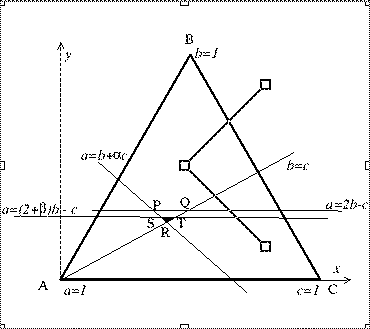
Figure 1
Thus, if we assume a uniform distribution, the probability of this type of
monotonicity failure is the ratio of the area of the small triangle (either
PQR or STR, whichever is the smaller) to the area of the large one (ABC). To
see why we must take the smaller triangle, note that to satisfy condition
M3, a point in Figure 1 must be below both the lines:
a = (2 + beta)b - c and a= 2b -
c.
Note that if beta > alpha, conditions M1-M3 cannot
simultaneously be satisfied, so in this case we define: Area (STR) = 0.
Switching to Cartesian coordinates,
x = c + b/2
y = sqrt(3) × b/2
the areas of the three triangles are found to be:
Area(ABC) = sqrt(3)/4
Area(PQR) =
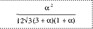
Area(STR) =
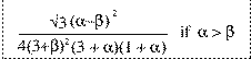
= 0 otherwise
So if we let p be the probability of monotonicity failure, we can
find its value as follows:
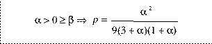
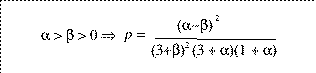
else p=0
Or, by substituting,
gamma = max{alpha, beta, 0}
delta = max{min{alpha, beta}, 0}
we obtain a single equation for p:
(P1) 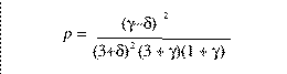
3. Estimating the transfer patterns
Clearly we need to know the likely pattern of transfers between candidates
from different parties, which requires access to the ballot papers of a
typical British electorate voting by STV for real political parties. Last
year an ERS/MORI exit poll of 3,983 London voters was conducted during the
European Parliament elections, in which they were asked to cast preferential
votes in two multi-member constituencies. The results form by far the best
available data on the likely behaviour of British voters in an election
conducted by STV.
Details of the poll may be found in Reference 3, which includes tables of
terminal transfers (transfers of votes from a candidate whose party has no
further candidates left who are still eligible to receive votes).
Unfortunately, there is no terminal data from Conservative candidates, since
none occurred in the count of the mock vote, so this data cannot be used.
Instead I try to consider all the possible transfers of votes which could
have taken place. For each of the two constituencies (London North and
London South), and for every ordered triple of candidates (Conservative,
Labour, Lib Dem), the following data extracted from the poll results is
used.
The number of votes which would transfer to the Labour candidate (if the
Conservative were to be eliminated leaving only the Labour and Lib Dem
candidates); the number which would transfer to the Lib Dem candidate in
such circumstances; and the number which would be non-transferable.
This data is repeated for the each of the Labour and Lib Dem candidates
being eliminated, providing 840 data sets (sadly not independent!) on which
to base the estimate of transfer patterns, and hence estimate p. The
number of data sets arises from 216 ordered triples in London North
(6-seater), 64 in London South (4-seater), and three data sets for each
ordered triple.
4. Method
In outline, I employ the following method (using an Excel spreadsheet):
- i) For each data set (representing the potential transfers from one
candidate from one party to two candidates from the other parties), the
proportions Tij of votes transferred to each of the surviving
candidates are calculated.
- ii) These proportions are then adjusted using the following approximate
shrinkage equation:
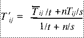
where:
- T 'ij represents the shrunken estimate of the proportion of
i's votes which transfer to j if i is eliminated.
- T-bar ij is the weighted sample mean of Tij based on
exclusions of candidates from the same party in a particular constituency.
- s is the sample variance of Tij.
- n is the size of the data set (the number of first preferences
credited to the excluded candidate).
- t = 0.0004
Note that this is based on a two-stage hierarchical model, in which (for a
given constituency and party) there is a party mean value of Tij,
with variance 0.0004, about which the candidates' Tij values are
distributed.
- iii) Based on the values of T 'ij, gamma, delta
and p are calculated, using the above definitions and equation P1.
- iv) For each ordered triple of candidates, the three values of
p (one for each potential elimination) are summed to allow for all
the possible ways in which monotonicity might fail, giving a total
probability P.
- v) For each constituency, a weighted mean of the probabilities is
calculated.
- vi) Finally a weighted mean of the probabilities for the two
constituencies is taken to produce the result:
E(P) = 2.5 × 10**(-4).
So, if the UK is divided into 138 multi-member constituencies, as proposed
in Reference 4, and assuming an average of one General Election every four
years, we would expect one instance of final-stage monotonicity failure
affecting party standing under STV roughly every 115 years.
5. Justifying the approach
The problem of estimating the probability of monotonicity failure under STV
is complicated, involving political considerations and statistical judgement
as well as pure mathematics. So inevitably I have had to make a number of
assumptions and simplifications. I will now attempt to identify all the
potential objections to my approach and answer some of the possible
criticisms.
5.1 Only monotonicity failure affecting parties is considered.
It is almost certainly true that the probability of affecting individual
candidates within a party is much greater. For a start, far more voters are
prepared to transfer within a party than between parties. This is supported
if we look at ERS Council Elections (which are like elections between
candidates of the same party since all support electoral reform), where
potential instances have been observed.
Nevertheless, given that STV is the only system which even attempts to
represent intra-party opinion, any minor 'imperfection' in this respect is
irrelevant to the choice of an electoral system. And it is certainly the
case that most of the opponents of STV are far more concerned with party
representation.
Finally, it is a necessary simplification since intra-party transfer
patterns are notoriously unpredictable and difficult to model.
5.2 The model only covers three parties and final-stage transfers.
Of course, earlier stages and a greater number of parties allow more
opportunities for monotonicity failure. However, I claim that the
probability of this making a difference to the final result is tiny compared
to the figure I have calculated above.
To see this, consider the diagram in figure 1. The effect is only possible
when there are three candidates with very similar votes (Q is the geometric
centre). Thus, if there are four candidates competing for the final place, a
candidate who 'benefits' in the penultimate stage is still very unlikely to
benefit in terms of election (and one who 'loses' probably would not have
been elected anyway).
If there are four candidates competing for two places, with three in danger
of elimination, then the fourth may be discounted (as a certainty), and we
are back to the original problem. Only in the case where there are four or
more candidates all with similar votes might a relevant situation arise; it
is reasonable to ignore such nth order terms.
5.3 The method assumes a Uniform (prior) distribution of votes between
the three parties.
This assumes that the three parties each have the same marginal
distribution. In a one-member constituency this is highly unlikely, but in a
multi-member constituency the relevant distribution to consider is the
remainder, once n-1 seats have been 'allocated', and the appropriate
number of quotas deducted from each party's vote.
Therefore, in order for the assumption to be reasonable, all we need is to
have across the country three parties capable of achieving proportions of
votes over a range of at least one quota. This would typically be achieved
by a party receiving 10% or more of the national (or regional) vote.
A similar principle is at work behind the Wichmann-Hill pseudo-random
generator, where the sum of a number of variables is known to tend to
normality, but the fractional part of the sum remains rectangular. There is
room here for someone to conduct a proper analysis, which I am confident
would uphold my assumption.
5.4 The results are based on an opinion poll conducted only in
London.
This represents probably the biggest area of doubt about the result and,
since this is the best data available so far, there is no way of avoiding
it. The STV ballot paper was constructed by listing (nearly) all candidates
in each of the Euro-constituencies represented. Since this was an election
for MEPs, recognition of most individual candidates must have been
relatively low.
However, we can only speculate on how voters would react in a General
election conducted by STV, and it is by no means obvious that voting
patterns would be substantially different. The same applies to the London
factor. While the relative positions of the parties would vary across the
country, there is no reason to suppose that the nature of voting patterns
would be any different.
5.5 Why has shrinkage been applied in this way?
Shrinkage is one of the results of Bayesian analysis which has been accepted
by non-Bayesian statisticians as representing a true effect which does not
appear in more traditional models. I have judged that a hierarchical model
is relevant to this situation, so we must take account of shrinkage. A
reference will be given in the next issue of Voting matters to
provide an explanation of shrinkage for non-statisticians.
If the charge is that I have not defined a full Bayesian hierarchical model,
with detailed multivariate prior distributions etc., then I plead guilty.
This was done deliberately to avoid specifying prior distributions which
might obscure the argument. The value of t is arbitrary but, I
believe, reasonable. A little sensitivity analysis shows that it does not
affect the final result by more than a tenth.
5.6 The weightings used in the final calculation do not allow for some
votes having a greater effect.
Rather than try to work out what effect the voting patterns might have had
in this particular election, I wanted to gain an estimate of overall voting
patterns. This means considering both first and last place candidates, since
in different constituencies each party will have somewhere between 0 and 5
'safe' seats, so the candidate involved in a three-way battle could be
anyone between the first and sixth most popular in that party.
The best way to cope with such uncertainty is to assign equal weightings to
each elector.
6. Conclusions
Using the best data available and using reasonable assumptions I have
estimated the probability that monotonicity failure would arise in a UK
General Election conducted by STV. That probability turns out to be
extremely small. In political terms it may as well be zero. Opponents of STV
will need to come up with better reasons if they wish to reject it out of
hand.
Acknowledgements
I am grateful to Professor Shaun Bowler of the University of California at
Riverside for his help in supplying data from the ERS/MORI poll, and to
Richard Wainwright and others for their encouragement and interest in this
research.
References
- Crispin Allard, 'Lack of Monotonicity - Revisited',
Representation 33:2 (1995), pp48-50.
- G. Doron and R. Kronick, American Journal of Political
Science 21, pp303-311.
- Shaun Bowler and David M. Farrell, 'A British PR
Election: Testing STV with London's Voters', Representation 32:120
(1994/5), pp90-3.
- Robert A. Newland, Electing the United Kingdom
Parliament, 3rd Edition (ERS, 1992).
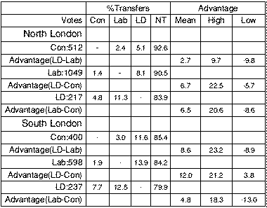
Appendix: Summary Statistics
Below is a table showing the transfer trends in North and South London. The
transfers are weighted means, expressed as percentages of the respective
first preference votes. The advantages (corresponding to alpha or
beta) are given after adjusting for shrinkage. See section 4 for a
full explanation. Each party is shown with the number of first preference
votes cast in the poll for candidates of that party.
Of the 3,983 voters polled, 3,013 expressed a valid first preference for a
candidate from one of the three main parties, of whom 1,778 were from North
London and 1,235 from South London. The overall probabilities of
monotonicity failure were found to be 0.00013 in North London and 0.00043 in
South London, giving a (weighted) mean of 0.00025 and a sample variance of 2
× 10**(-8).
Up: Issue 5
Next: Paper 2